Why pressure drop doesn’t always follow the square of flow: Lessons from six fittings
Est. Reading: 5 minutes
Why pressure drop doesn’t always follow the square of flow: Lessons from six fittings 3
Ask any engineer how pressure drop scales with flow rate and the answer comes back without hesitation. The square. Double the flow and you quadruple the loss. It is one of the first things anyone learns about piping, and most of us carry it for an entire career without ever putting a manometer on it.
Put eight manometers on a bench friction rig and check. Six fittings, each read separately at the same flow: the measured exponents come out at 1.03, 1.17, 1.21, 1.32, 1.37 and 1.81. Not one of them is 2.
Nothing is wrong with the rig, the fittings, or the textbook. The rule is simply being applied outside the conditions it was written for, and a bench apparatus is the cheapest place to find that out.
The Square Law Belongs to a Regime You Are Not In
The familiar relationship assumes fully developed turbulent flow, where the friction factor has stopped changing with Reynolds number and the loss is left varying with velocity squared. Laboratory flow rates do not get anywhere near that. At 1.00 gpm through the 13.6 mm bore of this apparatus the mean velocity is 0.434 m/s and the Reynolds number is about 5,900 — barely past the end of transition [1][2].
In that region even a perfectly smooth straight pipe will not give you an exponent of 2. The Blasius correlation puts the friction factor at 0.316 Re⁻⁰⋅²⁵, which makes pressure drop vary with flow to the power of about 1.75 rather than 2 [2][3]. A bend or a contraction, where the stream separates from the wall and has to reattach, departs further still. The gentlest of the three radius bends on this rig, the 150 mm one, fits an exponent of 1.03 across the working range — near enough to linear that a square-law estimate would be wrong by a factor of two at the top of the range.
The ranking is not intuitive either. The 90° mitre bend costs about thirty percent more than the smooth 90° elbow at the same flow, and among the three radius bends the sharpest beats the gentlest by nearly a third — differences of the sort that get rounded away in a design margin, visible side by side on the manometer bank in Figure 1.
Why pressure drop doesn’t always follow the square of flow: Lessons from six fittings 4
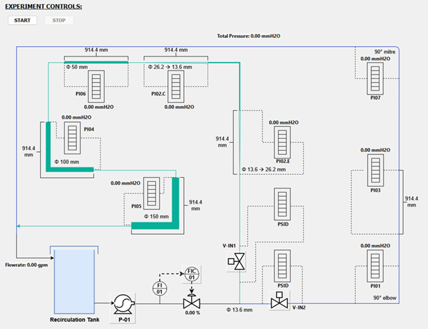
Figure 1. PiDeltaP process diagram — the two pipe networks, the eight manometer tappings with their fitting dimensions, and the FIC-01 flow controller.
The Fitting That Reads Small and Is Not
The clearest trap on the apparatus is a pair of fittings that are the same geometry run in opposite directions. At 1.00 gpm the sudden contraction from 26.2 mm down to 13.6 mm reads 35.2 mmH₂O. The sudden enlargement from 13.6 mm back up to 26.2 mm reads 3.8 — around a ninth of it.
The tempting conclusion is that an enlargement is nearly free. It is not. Its expansion loss coefficient is 0.534, which at that flow rate is 5.1 mmH₂O of head genuinely and irrecoverably lost. The tapping reads 3.8 because the stream is decelerating into the wider bore at the same time, handing back about 8.9 mmH₂O of velocity head as static pressure. What the manometer shows is the net of the two, and it is a measured pressure difference rather than an energy loss [4][5].
That distinction is a footnote in most courses. Read against the contraction, at the same flow, on the same bank of tubes, it stops being a footnote.
Eight Tappings, Two Routes, One Pump
PiDeltaP is a real-time simulator of the bench-top fluid friction apparatus that sits in unit operations laboratories. Water leaves the recirculation tank, is raised in pressure by pump P-01, is measured by flow element FI-01 and controlled by the control valve, and is delivered to a header that splits into two pipe networks. Everything after the pump is that pressure being spent, fitting by fitting, until what is left returns to the tank.
One network carries a 90° elbow, a straight 914.4 mm run of 13.6 mm bore pipe, and a 90° mitre bend. The other carries the sudden enlargement, the sudden contraction, and three bends of 50, 100 and 150 mm radius. Eight tappings read in millimeters of water, each one its own fitting, which is what makes them comparable.
The straight pipe is the exception, and deliberately so. Rather than being fitted to rig data like the other six, it is computed from the Darcy-Weisbach equation with the Blasius friction factor — so the one tapping where first principles are reliable is the one calculated from first principles, and it is there to be checked against [1][6].
Flow is set manually or automatically by the FIC-01 controller, and PID tuning set stays editable while the rig is running, so the same apparatus doubles as a flow control tuning exercise.
Open Both Valves and Let the Networks Negotiate
With one inlet valve open, all the measured flow goes that way and the other bank reads zero. Open both and the two networks are in parallel, and how the water divides between them is not something anybody gets to choose.
Run at 1.00 gpm through each route on its own and the elbow-and-mitre network totals 139.5 mmH₂O while the enlargement-and-bends network totals 180.1 — so the five-fitting route is the harder one. Open both and the simulator searches at every step for the pair of branch flows that makes the two pressure drops equal while still adding up to the measured total, exactly as the physical apparatus settles it. The higher-resistance route takes the smaller share, and you watch the balance establish itself instead of deriving it [1][6].
Operating either valve also injects a small flow transient, which with the controller in automatic is a free disturbance-rejection test on the same rig.
The File Holds Readings, Not Results
Every run exports to a timestamped CSV: elapsed time, which valves are open, the total flow, the total pressure and all eight individual manometers. What it does not contain is a single finished answer. There is no loss coefficient, no friction factor, no Reynolds number and no exponent anywhere in the file.
Those are the work, and they are what the lab report asks for. Plot pressure drop against flow on log-log axes across a range of flow rates and read the exponent off the slope of your own line. Work back from a measured drop and a known flow to the loss coefficient of the fitting, rather than looking it up in a table and trusting it [4][7].
Conclusion
Students come away with a coefficient they measured instead of one they were handed, and with a useful suspicion of a rule of thumb they were about to carry for thirty years. Instructors get a fluid mechanics experiment an entire cohort can run at once, against results that compare directly with the physical rig. Engineers get somewhere to find out what a restriction actually costs before it is welded in.
To request a demonstration of PiDeltaP and the full PiControl laboratory simulator portfolio, contact info@PiControlSolutions.com or visit www.picontrolsolutions.com.
References
[1] McCabe, W.L., Smith, J.C., and Harriott, P., Unit Operations of Chemical Engineering, 7th ed., McGraw-Hill, New York, 2005, Chapter 5: Flow of Fluids in Pipes and Thin Channels.
[2] White, F.M., Fluid Mechanics, 7th ed., McGraw-Hill, New York, 2011, Chapter 6: Viscous Flow in Ducts.
[3] Blasius, H., “Das Ähnlichkeitsgesetz bei Reibungsvorgängen in Flüssigkeiten,” Forschungsheft 131, VDI, Berlin, 1913.
[4] Crane Co., Flow of Fluids Through Valves, Fittings and Pipe, Technical Paper No. 410, Crane Co., Stamford, 2013.
[6] Perry, R.H. and Green, D.W. (Eds.), Perry’s Chemical Engineers’ Handbook, 9th ed., McGraw-Hill, New York, 2019, Section 6: Fluid and Particle Dynamics.
[7] Moody, L.F., “Friction Factors for Pipe Flow,” Transactions of the ASME, Vol. 66, 1944, pp. 671-684.